SVM with grid search parameters...
- Federico Nutarelli

- Jan 22, 2024
- 6 min read
Updated: Feb 29, 2024
Hi all, and welcome to this new post.
Today I would like to talk about Support Vector Machine, aka SVM.
In short, SVM is a supervised (i.e. you need to have the true labels in order to perform it) machine-learning method that seeks to find the optimal hyperplane (a plane in n dimensions) that maximizes the margin between different classes in the feature space. The SVM performs classification by constructing a hyperplane (or a set of hyperplanes)
in a high or even infinite-dimensional space, which can be used for both linear and non-linear classification.
A very informative series of videos about it is provided below:
Stealing from the internet, you may have noticed a lot of pictures like this for SVM:
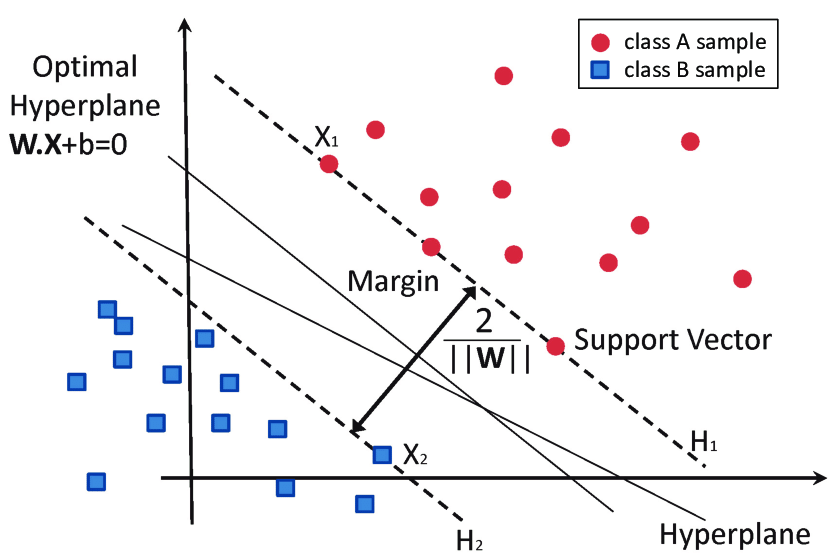
Support vectors are a key concept in the world of SVM. To understand support vectors, let's step back on SVM and first think of SVM as a method used for classification tasks – like deciding whether an email is spam or not. Imagine you have a bunch of points plotted on a graph. These points belong to two different categories (say, spam and not spam).
Basically, SVM's job is to find a line (or in more complex scenarios, a plane or a hyper-dimensional surface) that best separates these two categories.
This line is like a boundary: points on one side belong to one category (not spam), and points on the other side belong to another (spam).
Now, support vectors are the critical elements of this plot. They are the points that are closest to the separating line or boundary. Think of them like the frontier guards of each category. They are the ones that directly influence where the boundary lies. If these points were to move, the position of the line separating the categories would also change.
Specifically, in the context of the SVM, the data points that are closest to the hyperplane (support vectors) are the most critical elements of the dataset as they define the so-called margin. The effectiveness of the SVM in various applications is largely due to its reliance on kernel functions, which enable the method to operate in a transformed feature space without the need to compute the coordinates of the data in that space explicitly. This makes the SVM particularly suitable in handling high-dimensional
data and data for which the relationship between the class labels and attributes is not linearly separable.
The SVM's ability to manage overfitting through the regularization parameter makes it robust in various scenarios, especially in cases in which the dimension of the feature space exceeds the number of samples.
Kernels
Kernels in SVM are a bit like translators who help in understanding complex languages. When SVM faces a complex problem, where the data points are not easily separable by a straight line, kernels come into play.
Think of it this way: you have a bunch of points scattered on a flat table (a 2D plane), and you need to separate two types of points, say apples and oranges. If you can draw a straight line on the table to separate them, great! But what if you can't? This is where kernels step in. They take those points and lift them into a higher dimension - like picking them up from the table and floating them in the air, arranging them in such a way that you can now draw a simple plane (or a line) to separate the apples from the oranges.
In simpler terms, kernels transform complex, nonlinearly separable data (where a simple line can't do the job of separation in the original space) into a higher dimension where they become linearly separable (where you can easily draw a line or a plane to separate them).
Examples of kernels include:
Linear Kernel: This is the simplest form, used when the data is already linearly separable. It's like drawing a straight line or a flat plane.
Polynomial Kernel: It transforms the data into a higher dimension in a polynomial way (like curving the space). It's useful when the relationship between the variables is more complex than a straight line.
Radial Basis Function (RBF) Kernel: Also known as the Gaussian kernel, this is like creating a series of hills and valleys, where each point creates a hill. It's particularly effective for scenarios where the data points form clusters.
Sigmoid Kernel: Similar to the function used in neural networks, this kernel is like a complex curve that separates the points.
Each kernel has its own way of transforming the data, and choosing the right one depends on the specific problem you're dealing with. It's like choosing the right translator for a complex foreign language; the better the translation, the easier it is to understand and separate the data points (or in our analogy, the apples from the oranges).
Grid search
Grid Search in SVM is a powerful tool for optimizing the performance of your model. It systematically works through multiple combinations of parameter values, cross-validating as it goes to determine which tune gives the best performance.
Benefits of Grid Search in SVM:
Optimized Performance: By trying out a range of values for parameters like 'C' (regularization parameter) and 'gamma' (kernel coefficient), Grid Search helps in identifying the combination that maximizes the model's performance.
Automation of Hyperparameter Tuning: Instead of manually tweaking the parameters, Grid Search automates this process, saving time and reducing the risk of missing the optimal settings.
Cross-Validation Integration: It often integrates cross-validation, testing each parameter combination on different subsets of the data to ensure robustness, which helps in preventing overfitting.
Comprehensive Search: It explores a defined grid of parameters thoroughly, providing a more exhaustive search than manual or random searches.
Necessity of Grid Search:
Complexity of SVM Parameter Space: SVMs have a sensitive dependence on the correct setting of hyperparameters. Slight changes can significantly affect the model's performance, making a thorough search necessary.
No One-size-fits-all Solution: Different datasets require different parameter settings for optimal performance. Grid Search caters to this by exploring a wide range of possibilities.
Mock Example:
Let's say you're working with environmental data to predict air quality levels in various cities across different year ranges. Your SVM model has two main parameters to tune: 'C' and 'gamma'.
You perform Grid Search across multiple cities and year ranges. For each combination of city and year range, you read the corresponding datasets, preprocess them, and then apply Grid Search with a parameter grid defined as 'C': [0.1, 1, 10, 100], 'gamma': ['scale', 'auto']. The Grid Search uses cross-validation (cv=5) and is set to optimize the 'f1_weighted' score.
After running Grid Search, you collect the best parameters for each city-year pair. You then compute the average of the 'C' parameter and the most frequently occurring 'gamma' value across all city-year pairs. This gives you an idea of the general trend in optimal parameters for different datasets, which can be insightful for understanding the behavior of your model across diverse conditions.
Such an approach can be highly beneficial in practical applications where you deal with varied datasets requiring a nuanced understanding of how different SVM parameter settings affect the model's performance.
This is exactly what we did in our latest paper on urban competitiveness. If you are curious about a practical application stay tuned for the latest version!
If you're interested in seeing some code, here it is. We will attempt to apply a concept similar to honesty, though not exactly the same, by dividing our sample data, which spans from 2000 to 2014, into segments. Our goal is to predict data for the year t+5 using data from year t. To do this, we plan to split the data into pairs of five-year intervals. We will then learn the hyperparameters (within the specified range in the grid) using these pairs: 2000-2005, 2001-2006, 2002-2007, and so on, up to 2008-2013, as our training data. Afterwards, we'll use these learned hyperparameters to predict the data for 2014 using the data from 2009. This last part is not displayed. Specifically, for the sake of coherence with the above discussion, the code stops at the point where the optimal hyperparameters, `avg_gamma` ` avg_C`, are learned.
from sklearn.model_selection import GridSearchCV
from sklearn.svm import SVC
from sklearn.metrics import f1_score, roc_auc_score
from sklearn.model_selection import train_test_split
import pandas as pd
import numpy as np

# Define the parameter grid

param_grid = {
    'C': [0.1, 1, 10, 100],
    'gamma': ['scale', 'auto'],
    # Add other parameters here as needed
}

# Dictionary to hold the best hyperparameters for each city and year range
best_params_all = {}

# Loop over the cities and year ranges to read the datasets and perform grid search
for city in cities:
    best_params_all[city] = {}
    for year_range in year_ranges:

        # Reading datasets for each city and year_range
        # Replace file paths with actual file locations
        file_paths = [f'/file_path/thresholded_data/{city}{min(year_range)}.csv', f'/file_path/thresholded_data/{city}{max(year_range)}.csv']
        df_t = pd.read_csv(file_paths[0], header=None)
        df_t5 = pd.read_csv(file_paths[1], header=None)

        # Convert non-zero to 1 and keep zero as is
        df_t = df_t.applymap(lambda x: 1 if x > 0 else 0)
        df_t5 = df_t5.applymap(lambda x: 1 if x > 0 else 0)

        # Transpose and separate Y from X
        df_t_transposed = df_t.T
        df_t5_transposed = df_t5.T
        y = pd.Series(df_t_transposed.iloc[:, 0].values)
        X = df_t_transposed.iloc[:, 1:].values
        y_toverify = pd.Series(df_t5_transposed.iloc[:, 0].values)
        X_toverify = df_t5_transposed.iloc[:, 1:].values

        # Split data
        X_train, X_test, y_train, y_test = train_test_split(X, y, test_size=0.35, random_state=42)
        y_test5 = y_toverify.iloc[y_test.index]

        # Create a GridSearchCV object
        grid_search = GridSearchCV(SVC(probability=True, random_state=42), param_grid, cv=5, scoring='f1_weighted')
        grid_search.fit(X_train, y_train)

        # Save the best hyperparameters for the current city and year range
        best_params_all[city][year_range] = grid_search.best_params_

# Now, calculate the average of the best hyperparameters across all city-year pairs

avg_C = np.mean([params['C'] for city in best_params_all for params in best_params_all[city].values()])

avg_gamma_values = [params['gamma'] for city in best_params_all for params in best_params_all[city].values() if isinstance(params['gamma'], (int, float))]

avg_gamma = np.mean(avg_gamma_values) if avg_gamma_values else 'scale'
If you have questions, something is not clear, or you simply liked the post please feel free to leave a comment below! And don't forget the like :)
Comments